Q-Learning Explained with simple example
Reinforcement Learning
Tutorial
Artificial Intelligence
Machine Learning
A simple, easy to understand and step by step tutorial on Q-Learning using a simple example.

What is Q-Learning?
Q-learning is a model-free, value-based reinforcement learning algorithm. An agent learns to choose actions in a discrete environment to maximize cumulative rewards. It maintains a Q-table of estimates:
\(Q(s,a)\) = expected total reward starting from state s, taking action a, and thereafter following the optimal policy.
Key concepts
- State (s): represents the agent’s current situation (e.g., a grid cell).
- Action (a): a move available from a state, here Right (→) or Down (↓).
- Reward (r): immediate feedback after taking an action (−1 or +10).
- Learning rate (α): how quickly new information overrides old (here 0.5).
- Discount factor (γ): how much future rewards matter (here e.g. 0.9).
- Exploration rate (ε): probability of choosing a random action to explore (here e.g. 0.1).
Q-learning update rule:
Q(s,a) ← Q(s,a) + α · [ r + γ · maxₐ′ Q(s′,a′) − Q(s,a) ]Where:
- s = current state
- a = action taken
- r = reward received
- s′ = next state
- α = learning rate (0.5)
- γ = discount factor (0.9)
- maxₐ′ Q(s′,a′) = estimated best future value
Simple Example: 3×3 Grid World
Our environment is a 3×3 grid of states S00–S22:
| S00 (start) | S01 | S02 |
| S10 | S11 | S12 |
| S20 | S21 | S22 (goal) |
- Start at S00
- Goal at S22
- Reward = −1 per step, +10 upon reaching S22
- Valid moves: only → or ↓
Initial Q-table (Episode 0)
All Q-values start at 0. Invalid moves are shown as “—”.
| State | Q(→) | Q(↓) |
|---|---|---|
| S00 | 0 | 0 |
| S01 | 0 | 0 |
| S02 | — | 0 |
| S10 | 0 | 0 |
| S11 | 0 | 0 |
| S12 | — | 0 |
| S20 | 0 | — |
| S21 | 0 | 0 |
| S22 | — | — |
What is an Episode?
An episode is one full run from the start state S00 until the goal state S22:
Reset environment: agent begins at state S00.
Loop until the agent reaches S22 (goal):
- Select action via ε-greedy (ε=0.1).
- Move, observe reward (−1 or +10) and new state.
- Update Q(s,a) using the rule above.
Terminate when S22 is reached.
Record the Q-table snapshot after this episode.
Next episode: environment resets to S00, but Q-table retains learned values.
Over many episodes, Q-values propagate back from the goal so the agent learns the optimal path.
Episode 1 Walkthrough
After Episode 1, the Q-table is:
| Epi | State | Q(state →) | Q(state ↓) |
|---|---|---|---|
| 1 | S00 | –0.50 | NA |
| 1 | S01 | –0.50 | NA |
| 1 | S02 | NA | –0.50 |
| 1 | S10 | 0.00 | 0.00 |
| 1 | S11 | 0.00 | 0.00 |
| 1 | S12 | NA | 5.00 |
| 1 | S20 | 0.00 | NA |
| 1 | S21 | 0.00 | 0.00 |
| 1 | S22 | NA | NA |
Step-by-step updates in Episode 1
State S00: Q=0 vs 0 ⇒ pick →
- Move to S01, reward r = –1.
- Δ = –1 + 0.9·0 – 0 = –1 → Q(S00,→)=–0.50
State S01: 0 vs 0 ⇒ pick →
- Move to S02, r = –1.
- Δ = –1 + 0.9·0 – 0 = –1 → Q(S01,→)=–0.50
State S02: only ↓ valid
- Move to S12, r = –1.
- Δ = –1 + 0.9·0 – 0 = –1 → Q(S02,↓)=–0.50
State S12: only ↓ valid
- Move to S22, r = +10.
- Δ = 10 + 0.9·0 – 0 = 10 → Q(S12,↓)=5.00
All Episodes
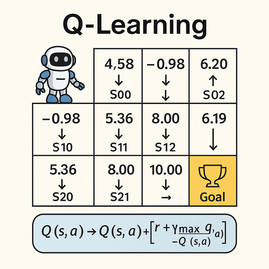
Final Q-Table (Episode 30)
Below is the Q-table snapshot after episode 30, showing the learned values converged from many trials:
| Episode | State | Q(state →) | Q(state ↓) |
|---|---|---|---|
| 30 | S00 | 4.58 | 1.65 |
| 30 | S01 | -0.98 | 6.20 |
| 30 | S02 | NA | 3.19 |
| 30 | S10 | 5.36 | -0.50 |
| 30 | S11 | 8.00 | 0.00 |
| 30 | S12 | NA | 10.00 |
| 30 | S20 | -0.50 | NA |
| 30 | S21 | 5.00 | NA |
| 30 | S22 | NA | NA |
Deriving the Optimal Policy
After 30 episodes, Q-values have converged. The greedy policy picks the action with the highest Q-value in each state:
π(s) = argmax_a Q(s,a)
| State | π(s) | Explanation |
|---|---|---|
| S00 | → | 4.58 > 1.65 |
| S01 | ↓ | 6.20 > -0.98 |
| S02 | ↓ | only ↓ is valid |
| S10 | → | 5.36 > -0.50 |
| S11 | → | 8.00 > 0.00 |
| S12 | ↓ | only ↓ is valid |
| S20 | → | only → is valid |
| S21 | → | only → is valid |
When the agent follows π(s) from S00, it will navigate optimally to S22 (goal).
Following the Learned Policy
Starting at S00, the agent moves according to π(s):
S00 --→--> S01 --↓--> S11 --→--> S12 --↓--> S22 (goal)This corresponds to the sequence of actions:
- S00 → S01
- S01 ↓ S11
- S11 → S12
- S12 ↓ S22
That’s the final, optimal route learned by Q-learning.
Summary
- Q-learning uses trial-and-error to learn optimal actions in a discrete environment.
- Learning rate α=0.5, discount factor γ=0.9, exploration ε=0.1 were used.
- Interactive pagination illustrates how Q-values evolve each episode.
- From converged Q-table, extract the greedy policy to guide the agent.
Earning Opportunity with AI
Grab Great Deals
Enjoyed this post?
If this article helped you,
☕ Buy me a coffee
Your support keeps more things coming!